Output Feedback (aka Pixels-to-Torques)
In this chapter we will finally start considering systems of the form: \begin{gather*} \bx[n+1] = {\bf f}(\bx[n], \bu[n], \bw[n]) \\ \by[n] = {\bf g}(\bx[n], \bu[n], \bv[n]),\end{gather*} where most of these symbols have been described before, but we have now added $\by[n]$ as the output of the system, and $\bv[n]$ which is representing "measurement noise" and is typically the output of a random process. In other words, we'll finally start addressing the fact that we have to make decisions based on sensor measurements -- most of our discussions until now have tacitly assumed that we have access to the true state of the system for use in our feedback controllers (and that's already been a hard problem).
In some cases, we will see that the assumption of "full-state feedback" is not so bad -- we do have good tools for state estimation from raw sensor data. But even our best state estimation algorithms do add some dynamics to the system in order to filter out noisy measurements; if the time constants of these filters is near the time constant of our dynamics, then it becomes important that we include the dynamics of the estimator in our analysis of the closed-loop system.
In other cases, it's entirely too optimistic to design a controller assuming that we will have an estimate of the full state of the system. Some state variables might be completely unobservable, others might require specific "information-gathering" actions on the part of the controller.
For me, the problem of robot manipulation is one important application domain where more flexible approaches to output feedback become critically important. Imagine you are trying to design a controller for a robot that needs to button the buttons on your shirt. Our current tools would require us to first estimate the state of the shirt (how many degrees of freedom does my shirt have?); but certainly the full state of my shirt should not be required to button a single button. Or if you want to program a robot to make a salad -- what's the state of the salad? Do I really need to know the positions and velocities of every piece of lettuce in order to be successful? These questions are (finally) getting a lot of attention in the research community these days, under the umbrella of "learning state representations". But what does it mean to be a good state representation? There are a number of simple lessons from output feedback in control that can shed light on this fundamental question.
Background
The classical perspective
To some extent, this idea of calling out "output feedback" as an
advanced topic is a relatively new problem. Before state-space and
optimization-based approaches to control ushered in "modern control", we
had "classical control". Classical control focused predominantly (though
not exclusively) on linear time-invariant (LTI) systems, and made very
heavy use of frequency-domain analysis (e.g. via the Fourier
Transform/Laplace Transform). There are many excellent books on the
subject;
What's important for us to acknowledge here is that in classical control, basically everything was built around the idea of output feedback. The fundamental concept is the transfer function of a system, which is a input-to-output map (in frequency domain) that can completely characterize an LTI system. Core concepts like pole placement and loop shaping were fundamentally addressing the challenge of output feedback that we are discussing here. Sometimes I feel that, despite all of the things we've gained with modern, optimization-based control, I worry that we've lost something in terms of considering rich characterizations of closed-loop performance (rise time, dwell time, overshoot, ...) and perhaps even in practical robustness of our systems to unmodeled errors.
From pixels to torques
Just like some of our oldest approaches to control were fundamentally solving an output feedback problem, some of our newest approaches to control are doing it, too. Deep learning has revolutionized computer vision, and "deep imitation learning" and "deep reinforcement learning" have been a recent source of many impressive demonstrations of control systems that can operate directly from pixels (e.g. consuming the output of a deep perception system), without explicitly representing nor estimating the full state of the system.
Imitation learning works incredibly well these days, even for very complicated
tasks (e.g.
Reinforcement learning (RL) definitely is solving difficult control problems,
though it currently still requires quite a bit of guidance (via cost function /
environment tuning) and requires an exhorbitant amount of computation.
Interestingly, it's quite common in reinforcement learning to solve a full-state
feedback problem first, and then to use "teacher student" (once again a form of
imitation learning) to distill the full-state feedback controller into an output
feedback control (e.g.
The synthesis of ideas between machine learning (both theoretical and applied) and control theory is one of the most exciting and productive frontiers for research today. I am highly optimistic that we will be able to uncover the underlying principles and help transition this budding field into a technology. My goal for this chapter is to summarize some of the key lessons from control that can, I hope, help with that discussion.
Static Output Feedback
One of the extremely important almost unstated lessons from dynamic programming with additive costs and the Bellman equation is that the optimal policy can always be represented as a function $\bu^* = \pi^*(\bx).$ So far in these notes, we've assumed that the controller has direct access to the true state, $\bx$. In this chapter, we are finally removing that assumption. Now the controller only has direct access to the potentially noisy observations $\by$.
So the natural first question to ask might be, what happens if we write our policies now as a function, $\bu = \pi(\by)?$ This is known as "static" output feedback, in contrast to "dynamic" output feedback where the controller is not a static function, but is itself another input-output dynamical system. Unfortunately, in the general case it is not the case that optimal policies can be perfectly represented with static output feedback. But one can still try to solve an optimal control problem where we restrict our search to static policies; our goal will be to find the best controller in this class to minimize the cost.
A hardness result
Let's consider the problem of designing a static output feedback for linear
systems (surely this should be the easy case!): $\dot\bx = \bA\bx + \bB\bu, \by =
\bC\bx.$ Unfortunately,
Parameterizations of Static Output Feedback
Consider the single-input, single-output LTI system $$\dot{\bx} = {\bf A}\bx + {\bf B} u, \quad y = {\bf C}\bx,$$ with $${\bf A} = \begin{bmatrix} 0 & 0 & 2 \\ 1 & 0 & 0 \\ 0 & 1 & 0\end{bmatrix}, \quad {\bf B} = \begin{bmatrix} 1 \\ 0 \\ 0 \end{bmatrix}, \quad {\bf C} = \begin{bmatrix} 1 & 1 & 3 \end{bmatrix}.$$ Here the linear static-output-feedback policy can be written as $u = -ky$, with a single scalar parameter $k$.
Here is a plot of the maximum eigenvalue (real-part) of the closed-loop system, as a function of $k.$ The system is only stable when this maximum value is less than zero. You'll find the set of stabilizing $k$'s is a disconnected set.

Just because this problem is NP-hard doesn't mean we can't find good controllers in practice. Some of the recent results from reinforcement learning have reminded us of this. We should not expect an efficient globally optimal algorithm that works for every problem instance; but we should absolutely keep working on the problem. Perhaps the class of problems that our robots will actually encounter in the real world is a easier than this general case (the standard examples of bad cases in linear systems, e.g. with interleaved poles and zeros, do feel a bit contrived and unlikely to occur in practice).
Perhaps a history of observations?
In addition to giving a potentially bad optimization landscape, it's pretty easy to convince yourself that making decisions only based on the current observations is not sufficient for decision making in all problems. Take, for example, the LQR controller we derived for balancing an Acrobot or Cart Pole -- these controllers were a function of the full state (positions and velocities). If our robot is only instrumented with position sensors (e.g. encoders), or if our observations are instead coming from a camera pointed at the robot, then by looking at only the instantaneous observations would not have any information about the joint velocities. Although it would have to be shown, it seems reasonable to expect that no controller of this form could accomplish the balancing task (even for the linearized system) from all initial conditions.
One common response today is: what if we make the controller a function of some finite recent history of observations? If there is no measurement noise, then the last two position measurements are sufficient to make a (slightly delayed) estimate of the velocity. If there is measurement noise, then taking a slightly longer history would allow us to filter out some of that noise. Yes! This is on the right track. Technically this would no longer be a "static" controller; it requires memory to store the previous observations and memory is the defining characteristic of a "dynamic" controller. But how much history/memory do we need?
Partially-observable Markov Decision Processes (POMDPs)
For an upper bound on the answer to the question "how much memory do we need?", we can turn to the key results from the framework of POMDPS. The short answer is that if we use the entire history of actions and observations, then this is clearly sufficient for optimal decision making. Rather than maintaining this expanding history explicitly, we can instead maintain a representation that is a sufficient statistic for this history. In the good cases, we can find sufficient statistics that have a finite representation.
A (finite) partially-observable Markov decision process (POMDP) is a stochastic
state-space dynamical system with discrete (but potentially infinite) states $S$,
actions $A$, observations $O$, initial condition probabilities $p_{s_0}(s)$,
transition probabilities $p(s'|s,a)$, observation probabilities $p_{o|s}(o | s)$, and
a deterministic cost function $\ell: S \times A \rightarrow \Re$
An important idea for POMDP's is the notion of the belief state of a POMDP: \[ b_i[n] = P(s[n] = s_i | a[0] = a_0, o[0] = o_0, ... a_{n-1}, o_{n-1}).\] ${\bf b}[n] \in \mathcal{B}[n] \subset \Delta^{|S|}$ where $\Delta^m \subset \Re^m$ is the $m$-dimensional simplex and we use $b_i[n]$ to denote the $i$th element. ${\bf b}[n]$ is a sufficient statistic for the POMDP, in the sense that it captures all information about the history that can be used to predict the future state (and therefore also observations, and rewards) of the process. Using ${\bf h}_n = [a_0, o_0, ..., a_{n-1}, o_{n-1}]$ to denote the history of all actions and observations, we have $$P(s[n+1] = s | {\bf b}[n] = {\bf b}_n, {\bf h}[n] = {\bf h}_n, a[n] = a_n) = P(s[n+1] = s | {\bf b}[n] = {\bf b}_n, a[n] = a_n).$$ It is also sufficient for optimal control, in the sense that the optimal policy can be written as $a^*[n] = \pi^*({\bf b}[n], n).$
The belief state is observable, with the optimal Bayesian estimator/observer given by the (belief-)state-space form as $$ b_i[n+1] = f_i({\bf b}[n], a[n], o[n]),$$ where $b_i[0] = p_{s_0}(s_i)$, and $$f_i({\bf b}, a, o) = \frac{p_{o|s}(o \,|\, s_i) \sum_{j \in |S|} p(s_i\,|\,s_j,a) b_j}{p_{o|b,a}(o \,|\, {\bf b}, a)} = \frac{p_{o|s}(o \,|\, s_i) \sum_{j \in |S|} p(s_i\,|\,s_j,a) b_j}{\sum_{i \in |S|} p_{o|s}(o \,|\, s_i) \sum_{j \in |S|} p(s_i | s_j, a) b_j}.$$ Using the transition matrix notation from MDPs we can rewrite this in vector form as $$f({\bf b}, a, o) = \frac{\text{diag}({\bf c}(o)) \, {\bf T}(a) \, {\bf b}}{{\bf c}^T(o) \, {\bf T}(a) \, {\bf b}},$$ where ${\bf c}(o)$ is the column vector with $c_i(o) = p_{o|s}(o \,|\, s_i).$ Moreover, we can use this belief update to form the ``belief MDP'' for planning by marginalizing over the future observations, giving the \begin{align*} p_{\text{bMDP}}({\bf b}'|{\bf b}, a) = \sum_{i \in |O|} p({\bf b}'| {\bf b}, a, o_i) p_{o |b,a}(o_i | {\bf b}, a) = \sum_{i \in |O|} p({\bf b}'| {\bf b}, a, o_i) {\bf c}^T(o_i) \, {\bf T}(a) \, {\bf b},\end{align*} where $p({\bf b}'| {\bf b}, a, o)$ is 1 if ${\bf b}' = f({\bf b},a,o)$ and 0 otherwise.
The belief MDP is a little scary -- we are evolving distributions over possible beliefs! Perhaps one small consolation is that for discrete problems, even though ${\bf b}[n]$ is represented with a vector of real values, it actually lives in a finite space, $\mathcal{B}[n]$, because only a finite set of beliefs are reachable in $n$ steps given finite actions and observations. The policy $\pi^*({\bf b}[n], n)$ which optimal state feedback for the belief MDP is exactly the optimal output feedback for the original POMDP.
The Cheeze Maze
One of the classic simple examples from the world of POMDPs is the "cheese
maze"
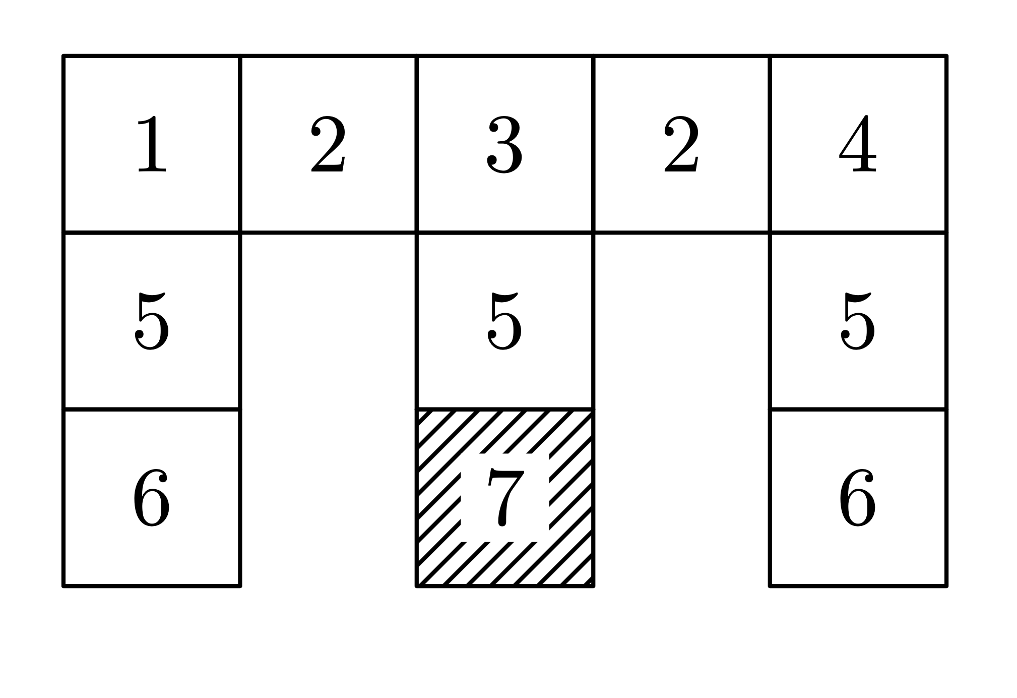
Imagine you are placed at a (uniform) random position in the maze. You do get to know the map, but you don't get to know your location. What would be your strategy for navigating to the goal? If your initial observation is 5, you have a decision to make... are you optimistic and try moving down (in the hopes that you'll find the goal?), or do you move up to see a 1, 3, or 4? What about if your initial observation is a 2?
One can write the optimal policy for this specific problem with exactly 7 discrete (belief) states. Can you find them?
It's not immediately clear how to losslessly represent distributions over possible beliefs (functions over $\Re^{|S|}$ in the finite state case), but it turns out that the value function has some known important properties...
More generally, in continuous state spaces, the belief state is a function ${\bf b}(\bx, n) = p_{x|h}(\bx[n] \,|\, {\bf h}[n]):$
There is a wealth of literature on POMDPs in robotics, and on POMDP solution techniques. See
Linear systems w/ Gaussian noise
Linear Quadratic Regulator w/ Gaussian Noise (LQG)
Trajectory optimization with Iterative LQG
Observer-based Feedback
Since we know so much about designing full-state feedback controllers, one of the most natural (and dominant) approaches to control is to first design an observer (aka "state estimator"), and then to use state feedback. Famously, this approach is actually optimal for the quadratic regular objective on linear-Gaussian systems (LQG) -- this is known as the "separation principle". But it is certainly not optimal in general!
Luenberger Observer
Disturbance-based feedback
There is an interesting alternative to trying to observe/estimate the true state
of the system, which can in some cases lead to convex formulations of the
output-feedback objective. The notion of disturbance-based feedback, which we introduced in the context of stochastic/robust
MPC, can be extended to disturbance-based output feedback:
\begin{gather*} \bx[n+1] = \bA\bx[n] + \bB\bu[n] + \bw[n],\\ \by[n] = \bC\bx[n] +
\bv[n], \end{gather*} by parameterizing an output feedback policy of the form
$$\bu[n] = \bK_0[n] \by[0] + \sum_{i=1}^{n-1}\bK_i[n]{\bf e}[n-i],$$ where ${\bf
e}[n] = ...$
Optimizing dynamic policies
Convex reparameterizations of $H_2$, $H_\infty$, and LQG
DGKF (solving two Riccati equations)
Scherer's convex reparameterizations of LQG
Policy gradient for LQG
Sums-of-squares alternations
Coming soon. See, for instance,
Teacher-student learning
Feedback from pixels
In my opinion, one of the most important advances in control in the last decade has been the introduction of high-rate feedback from cameras. This advance was enabled by the revolution in computer vision that came with deep learning. Especially in the domain of robotic manipulation, the value of this feedback is undeniable. Unfortunately, these sensors break many of the synthesis tools that we've discussed in the notes -- not only are they very high dimensional, but the space of RGB images is horrible and non-smooth. As of this writing, conventional wisdom is that model-based control does not have a lot to offer to this problem -- to design control from cameras, we are often limited to either imitation learning or black-box reinforcement learning. (I personally think that we have thrown the baby out with the bathwater, and consider a highly important research area to close this gap.)
More coming soon...